Logic and Computation

This video walks through the concepts on this page with live terminal demonstrations and auto-generated graph diagrams. Section links (🎬) throughout the page jump to the corresponding part of the video.

---

zelph is a logic programming system, but not in the traditional sense. Where Prolog operates on terms and Datalog on flat relations, zelph stores everything — facts, rules, predicates, even numbers — as structures in a single semantic network. Computation does not happen outside the graph; it emerges from the graph, through rule-driven inference over its topology.

This page introduces zelph's reasoning capabilities from a logic programming perspective. For the basic syntax of facts, sets, and lists, see Core Concepts. For a hands-on quick start, see the Quick Start Guide.

Positioning: Forward Chaining over Graphs

🎬 Watch this section

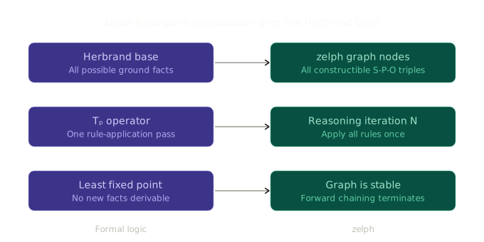
zelph's inference engine performs forward chaining (bottom-up evaluation), similar to Datalog or production rule systems. When a new fact is asserted or a rule is defined, the engine immediately checks whether any rule conditions are newly satisfied and derives all possible consequences. This process repeats until a fixed point is reached — no further facts can be derived.

This is fundamentally different from Prolog's top-down, goal-driven search with backtracking. zelph does not search for proofs; it materializes all derivable facts in the graph. In formal terms, this is a least-fixed-point computation over the graph's Herbrand base: start with the asserted facts, apply all rules to derive new facts, repeat until no iteration produces anything new. The trade-off is deliberate: forward chaining integrates naturally with knowledge graphs (where facts arrive incrementally, e.g. from Wikidata imports) and guarantees termination for Datalog-safe rules.

What sets zelph apart from both Prolog and Datalog is the representation: rules, predicates, and even the concept of conjunction are themselves nodes in the graph. This homoiconicity enables meta-reasoning, self-referential structures, and a seamless boundary between knowledge and computation.

The Executable Graph

🎬 Watch this section

A defining characteristic of zelph is its homoiconicity: logic (code) and facts (data) share the exact same representation.

In many traditional semantic web stacks (like OWL/RDF), the ontology is descriptive. For example, an OWL "cardinality restriction" describes a constraint, but the actual logic to enforce that constraint resides hidden in the external reasoner's codebase (e.g., HermiT or Pellet). The operational semantics are external to the data.

In zelph, the logic is intrinsic to the data.

• Rules are Data: Inference rules are not separate scripts; they are specific topological structures within the graph itself. The implication operator => is a standard relation node; the conditions form a set tagged as a conjunction — all represented by ordinary subject–predicate–object triples.
• Predicates are Nodes: Every relation type (including user-defined ones) is a first-class node in the graph, not an edge label. This means you can write rules about predicates — declaring symmetry, transitivity, or functional constraints as graph-level properties.
• Math is Data: Numbers are not opaque literals but Lisp-style cons-lists of digit nodes that interact with semantic entities through the same rule mechanism.

This means the graph doesn't just describe knowledge; it structures the execution of logic. The boundary between "data storage" and "processing engine" is effectively removed. Consequently, importing data (e.g., from Wikidata) can immediately alter the computational behavior of the system.

Relation Nodes and Self-Reference

Every fact in zelph — every subject–predicate–object triple — is represented by a dedicated relation node. This node can immediately serve as the subject, the object or the predicate of further facts, enabling statements about statements without any special mechanism.

A rule is such a fact too, so it can be talked about like any other — and talking about one does not claim it. Only the rule that was stated on its own fires; the one that is merely quoted is a part of the sentence quoting it:

zelph> (X p Y) => (X q Y)
zelph> ((X buys Y) => (X owns Y)) "was proposed by" alice
zelph> a buys car
zelph> a p b
(a q b) ⇐ (a p b)

a buys car derives nothing: alice's proposal is on record, not in force. Nothing has to be remembered for this — an asserted rule is a part of no other fact, a quoted one is the subject, the predicate or an object of the sentence that quotes it — so it survives .save and .load unchanged.

Predicate position is the least obvious of the three, and it works like the others:

zelph> a p b
zelph> x (a p b) y
zelph> X (a p b) Y
Answer: x (a p b) y

Anything used as a predicate becomes a relation type, so the composite predicate appears among them and the fact is found by a rule quantifying over predicates just like any other:

zelph> X Y Z
Answer: (a p b) ~ ->
Answer: p ~ ->
Answer: a p b
Answer: x (a p b) y

(abridged — the query also lists the core relation types). This holds independently of how the network came to be: a graph read back from a .bin answers exactly as the one that was typed.

A composite predicate may itself carry variables, and then it is a pattern like any other — it unifies structurally rather than being looked up by identity, so it reaches inside the predicate. In a query:

zelph> a p b
zelph> x (a p b) y
zelph> S (a P b) O
Answer: x (a p b) y

and in a rule, where the variables it binds are available to the consequence:

zelph> a p b
zelph> x (a p b) y
zelph> (S (a P b) O) => (P links S)
(p links x) ⇐ (x (a p b) y)
zelph> S links O
Answer: p links x

The same holds in a consequence: (X p Y) => (X (Y r s) c) derives a (b r s) c, and the instantiated predicate is declared a relation type like every other.

This is in contrast to RDF, where a triple is an edge with no inherent identity. To make a statement about a triple in classic RDF, you need reification: four additional triples that decompose and name the original one. The RDF-star extension was introduced specifically to address this limitation.

In zelph, this problem does not exist. Every statement is already a node. The relation node serves a purpose analogous to Gödel numbering — it makes the system self-referential by giving every statement a first-class identity within the system. But where Gödel had to route through arithmetic encoding (prime factorization), zelph's reification is structural: the node is the statement, with no encoding or decoding step.

Comparisons with Other Systems

🎬 Watch this section

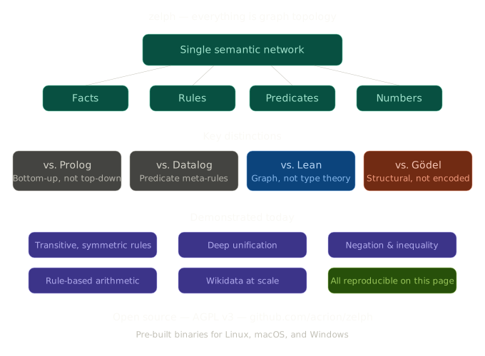
zelph's design can be understood through comparisons with several established systems. These comparisons highlight both shared principles and fundamental differences.

Prolog and Datalog

Prolog performs top-down, goal-driven search with backtracking. zelph performs bottom-up forward chaining, like Datalog: it materializes all derivable facts until a fixed point is reached.

But unlike standard Datalog, zelph's predicates are first-class nodes. This enables meta-rules — rules that quantify over relations themselves — which are impossible to express in standard Datalog and require meta-interpreters in Prolog.

Lean and Curry-Howard

🎬 Watch this section

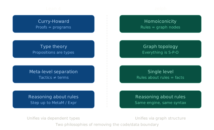
Lean 4 is a powerful theorem prover based on dependent type theory. Through the Curry-Howard correspondence, proofs in Lean are programs — propositions are types, and proofs are terms. This is a beautiful unification of logic and computation, but it is a different kind of unification than what zelph provides.

In Lean, the inference machinery — tactics, the elaboration pipeline, the MetaM monad — lives in a metaprogramming layer that operates on terms but is not itself expressed as terms in the same way. To reason about a proof as data, you step up to a meta-level (the Expr API).

In zelph, there is no meta-level. Rules, facts, predicates, and numbers all live in the same graph. A rule about a predicate is written in the same syntax, stored in the same structure, and processed by the same engine as any ordinary fact. The boundary between "data" and "logic" is removed entirely.

Lean unifies through type theory. zelph unifies through graph topology. These are philosophically very different approaches to the same goal: erasing the boundary between code and data.

Gödel Numbering

🎬 Watch this section

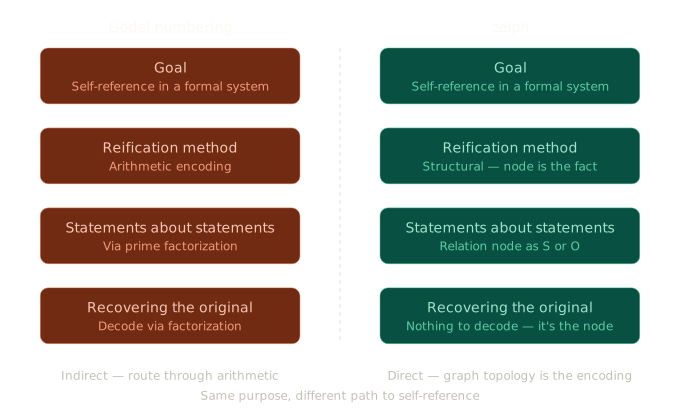
In 1931, Gödel showed that formal systems can reason about themselves by encoding formulas as numbers via prime factorization. Arithmetic statements about those numbers become, implicitly, statements about formulas.

zelph's relation nodes serve the exact same purpose: they make the system self-referential. Every statement gets a node, and that node can immediately participate in further statements. But where Gödel's encoding is arithmetic — requiring encoding and decoding via prime factorization — zelph's reification is structural. The node is the statement. No encoding, no decoding. It is a more direct path to the same goal: self-reference within a formal system.

Lisp and S-Expressions

🎬 Watch this section

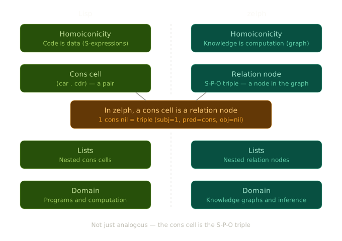
Lisp's famous "code is data" principle — homoiconicity via S-expressions — is a direct ancestor of what zelph does. But where Lisp applies this idea to programs via cons-cell lists, zelph applies it to knowledge via subject–predicate–object triples.

The connection goes deeper than analogy: zelph's lists are actual Lisp-style cons-lists built from cons and nil nodes, and a cons cell is a relation node (a triple with cons as the predicate). The S-P-O triple is zelph's equivalent of Lisp's S-expression — the universal data structure from which everything else is composed.

Rules Over Graphs

Basic Rules and Conjunction

🎬 Watch this section

A rule in zelph connects a set of conditions to a consequence via the => operator. The conditions form a conjunction: all must match simultaneously under a shared variable binding.

The idiomatic syntax uses commas to separate conditions:

(cond1, cond2, cond3) => consequence

Variables are single uppercase letters (A–Z) or identifiers starting with _ (e.g. _Var). They are scoped to the current rule and universally quantified: the rule fires for all bindings that satisfy the conditions.

Everything else is a name, and that includes multi-letter uppercase tokens such as DA or SUM. A rule that uses one as if it were a variable asks for that one specific node instead of binding anything, so it never fires — and it does so silently, which looks exactly like an engine that refuses to match. Write _DA when a longer variable name reads better.

A classic example — transitive closure:

zelph> (R is transitive, A R B, B R C) => (A R C)
zelph> > is transitive
zelph> 6 > 5
zelph> 5 > 4
(6 > 4) ⇐ {(6 > 5) (> is transitive) (5 > 4)}

After entering 5 > 4, the engine finds that the three conditions are jointly satisfiable with R = >, A = 6, B = 5, C = 4, and derives 6 > 4.

Several Consequences

A rule may conclude more than one thing at once. The consequences are written as several objects of the same rule. The comma is the conjunction of conditions; on the right-hand side it is refused with a message naming this form, rather than guessed at:

zelph> .deductions all
Deduction printing mode: all
zelph> (A is human) => (A has consciousness) (A has mortality)
zelph> tim is human
(tim has mortality) ⇐ (tim is human)
(tim has consciousness) ⇐ (tim is human)

The objects of a fact are an unordered set, so which of the two is announced first is not defined.

This is not the same as writing two rules with the same conditions. One rule fires once, so its consequences share their fresh variables: (X p Y) => (X q N) (N r Y) links X to a generated node and that same node to Y, while two separate rules would generate one node each.

Meta-Rules: Predicates as First-Class Nodes

🎬 Watch this section

Notice that R in the transitive rule is a variable ranging over predicates. This is possible because predicates in zelph are nodes, not edge labels. Any relation declared is transitive automatically benefits from this single rule — no separate rule per predicate is needed.

This enables a class of rules that are difficult or impossible to express in standard Datalog or Prolog: rules that reason about relations themselves.

Example — Symmetric relations:

zelph> (R is symmetric, X R Y) => (Y R X)
zelph> friend is symmetric
zelph> alice friend bob
(bob friend alice) ⇐ {(alice friend bob) (friend is symmetric)}

A single rule declares the semantics of symmetry for any relation. Declaring friend is symmetric is a fact about the predicate friend; the rule matches it and closes over all instances.

Example — Opposite relations:

zelph> (R "is opposite of" S, X R Y) => (Y S X)
zelph> "has part" "is opposite of" "is part of"
zelph> chimpanzee "has part" hand
(hand "is part of" chimpanzee) ⇐ {("has part" "is opposite of" "is part of") (chimpanzee "has part" hand)}

Declaring that "has part" is opposite of "is part of" causes every has part fact to automatically generate its inverse. The rule is generic: it works for any pair of opposite relations without modification.

Rules That Derive Rules

A consequence does not have to be a fact. It can be a rule — and then the outer rule is a rule schema: firing it writes a new rule into the graph, which the engine picks up and applies within the same run.

The inner rule's variables belong to the inner rule. Only what the outer rule's conditions bind is substituted; everything else comes through as a variable, so what arrives is a rule and not one instance of one.

Example — transitivity as a schema:

zelph> (R is transitive) => ((X R Y, Y R Z) => (X R Z))
zelph> before is transitive
(((Y before Z), (X before Y)) => (X before Z)) ⇐ (before is transitive)
zelph> a before b
zelph> b before c
(a before c) ⇐ {(b before c) (a before b)}
zelph> c before d
(a before d) ⇐ {(c before d) (a before c)}
(b before d) ⇐ {(c before d) (b before c)}

R was bound to before and is gone; X, Y and Z were bound by nothing and stayed variables. What the second line derives is the transitivity rule for before, and one such rule appears for every relation declared transitive.

Compare this with the meta-rule (R is transitive, X R Y, Y R Z) => (X R Z), which expresses the same closure by quantifying over the predicate at match time. The schema instead pays that quantification once, when the relation is declared, and leaves a specialised rule behind. Both are available; the schema is the one that can make the shape of a rule depend on data.

Example — a rule under a switch:

zelph> (K is on) => ((X p Y) => (X q Y))
zelph> a p b
zelph> A q B
zelph> k is on
((X p Y) => (X q Y)) ⇐ (k is on)
(a q b) ⇐ (a p b)
zelph> A q B
Answer: a q b

The inner rule is written out from the start and a p b is there before the switch, yet the query answers nothing until k is on arrives. That is not a scheduling accident, it is the next section.

Example — an ontology's property axioms as data:

Sub-property, domain and sub-class are the axioms an ontology is normally described with. Written once as schemas, every declaration a modeller makes afterwards is ordinary data — and produces its own rule:

zelph> .deductions all
Deduction printing mode: all
zelph> (P is transitive) => ((X P Y, Y P Z) => (X P Z))
zelph> (P subpropertyof Q) => ((X P Y) => (X Q Y))
zelph> (C subclassof D) => ((X isa C) => (X isa D))
zelph> (P domain C) => ((X P Y) => (X isa C))
zelph> mother subpropertyof parent
((X mother Y) => (X parent Y)) ⇐ (mother subpropertyof parent)
zelph> parent domain person
((X parent Y) => (X isa person)) ⇐ (parent domain person)
zelph> person subclassof agent
((X isa person) => (X isa agent)) ⇐ (person subclassof agent)
zelph> m mother n
(m parent n) ⇐ (m mother n)
(m isa person) ⇐ (m parent n)
(m isa agent) ⇐ (m isa person)

One statement of data, m mother n, walked three rules that nobody wrote — and each step carries its own justification, so .explain (m isa agent) reconstructs the chain back to it.

Rules that write rules have a page of their own: Rules That Write Rules covers where the idea comes from (it is the axiom schema of logic, with the instances made real), what happens when a generator matches many times, generators that generate generators, and the edges of the construct.

Mentioning a Rule Is Not Asserting It

Writing a rule down inside another statement talks about it; it does not claim it.

zelph> ((X p Y) => (X q Y)) is questionable
zelph> a p b
zelph> A q B
zelph>

Nothing fires — which is the only defensible reading, since the alternative is that doubting a rule puts it to work.

The distinction is decidable from the graph alone, and cheaply. Building a rule in order to talk about it creates the same nodes and the same edges as asserting it, so the rule node itself cannot say which happened — but its surroundings can: an asserted rule is a part of nothing, while a mentioned one is the subject, the predicate or an object of the statement that mentions it. Nothing is remembered, so a .save/.load round trip cannot lose the difference, and a graph without rules never pays for the test.

This is what makes the switch above work. Until k is on fires, (X p Y) => (X q Y) is an object of the outer rule and therefore a mention; firing the outer rule asserts a copy of it, which is a part of nothing and consequently live.

The one shape this cannot separate is a fully ground rule — no variables anywhere — that is asserted and mentioned at once: hash-consing makes those a single node. A rule with variables is two nodes, because every statement names its own variables.

Deep Unification

🎬 Watch this section

zelph's unification engine matches patterns against arbitrarily nested structures. This is essential for reasoning about statements-about-statements — a natural consequence of zelph's graph topology where fact nodes can themselves appear as subjects or objects of other facts.

zelph> .deductions all
Deduction printing mode: all
zelph> ((A + B) = C) => (test A B)
zelph> (4 + 5) = 9
(test 4 5) ⇐ ((4 + 5) = 9)

The rule's condition pattern ((A + B) = C) requires a fact whose subject is itself a fact matching (A + B). The engine recursively walks the graph topology, binding A = 4, B = 5, C = 9.

.deductions all is necessary here because the derived fact pertains to test, a node not referenced in the typed statement, so the default focus mode counts it instead of printing it – see Deduction Output Modes. (In test A B the variables occupy predicate and object position: the derived statement is test, related to 5 through the predicate 4.)

This extends to arbitrary depth:

zelph> .deductions all
Deduction printing mode: all
zelph> (subj pred (obj is (subj2 A (b test C)))) => (success A C)
zelph> subj pred (obj is (subj2 a_val (b test c_val)))
(success a_val c_val) ⇐ (subj pred (obj is (subj2 a_val (b test c_val))))

Deep unification also works within conjunction conditions, enabling rules that combine structural decomposition with multi-condition reasoning:

zelph> ((A + B) = C) => (test A B)
zelph> (4 + 5) = 9
zelph> (*{ ((A + B) = C) (B followed-by D) (C followed-by E) } ~ conjunction) => ((A + D) = E)
zelph> 5 followed-by 42
zelph> 9 followed-by 43
((4 + 42) = 43) ⇐ {((4 + 5) = 9) (5 followed-by 42) (9 followed-by 43)}

This rule decomposes the nested equation (A + B) = C, uses the bound values to look up successor relationships, and assembles a new equation — all in a single inference step.

What the conjunction tag decides, and what it does not

The tag says how the members of a condition container combine; it is not what makes the node a container. With more than one member it is the only thing that says so, and other combinations are conceivable — so an untagged container of several conditions is left alone rather than read as a conjunction.

A container of exactly one member is different: no combination of one thing can differ from any other, so the tag cannot change what the rule means. All four spellings below are therefore the same rule, and all four fire:

(X p Y) => (X q Y)                        # one condition, no container
{(X p Y)} => (X q Y)                      # written out in set notation
*{(X p Y)} => (X q Y)                     # ... with the focus operator
(*{(X p Y)} ~ conjunction) => (X q Y)     # ... and tagged explicitly

Facts with Multiple Objects

🎬 Watch this section

A fact in zelph connects a subject to an object via a predicate. When a fact has multiple objects (e.g. f maps 1 2), these objects form an unordered set — there is no defined ordering among them. The statement f maps 1 2 means: f is related via maps to both 1 and 2, but it does not encode which is "first" and which is "second".

This is a deliberate design choice: zelph's internal topology represents objects as a set of incoming connections to the fact node, not as a sequence.

When order matters — for example, to represent a mapping from a domain element to a codomain element — you must use lists (cons-lists via angle brackets <...>), which provide an explicit structural ordering. See Angle Brackets: Lists for details on the list syntax.

Example — unordered objects in rules:

zelph> alice parent_of bob charlie
zelph> (A parent_of B) => (B child_of A)
(bob child_of alice) ⇐ (alice parent_of bob)
(charlie child_of alice) ⇐ (alice parent_of charlie)

The rule matches each object independently. Whether bob or charlie was written first is irrelevant — both are equally "objects of" the parent_of fact.

This distinction becomes critical in more complex rules. Consider a naïve attempt at function composition using multiple objects:

(F maps A B, G maps B C) => ((G compose F) maps A C)
f maps 1 2
g maps 2 3

The engine cannot distinguish "domain" from "codomain" here, because both are unordered objects of the same fact: f maps 1 2 matches F maps A B with A = 1, B = 2 and equally with A = 2, B = 1. So the rule derives not only (g compose f) maps 1 3 but also (f compose g) maps 1 3, and each of those is itself a maps fact whose subject is a composite the rule has just built – which feeds the rule again, with ((f compose g) compose g), then (((f compose g) compose g) compose (g compose f)), and so on. The terms grow without bound and there is no fixed point to reach.

Do not type this one in. It is here as the mistake to recognize, not as an example to run: three lines are enough to make the engine derive until the session is ended from outside, since a run in progress cannot be stopped from the prompt.

Example — Function composition with lists:

🎬 Watch this section

The correct approach uses ordered lists to encode the domain–codomain relationship:

zelph> (F maps <A B>, G maps <B C>) => ((G compose F) maps <A C>)
zelph> f maps <item1 item2>
zelph> g maps <item2 item3>
((g compose f) maps <item1 item3>) ⇐ {(g maps <item2 item3>) (f maps <item1 item2>)}

The list <A B> is a cons-list with a defined structure: A is the first element (car) and B is the rest (cdr). Deep unification matches this structure precisely, so A unambiguously binds to the domain element and B to the codomain element.

The consequence (G compose F) creates a new fact node representing the composition, which then becomes the subject of maps. This is higher-order reasoning expressed as first-order graph topology — with the structural ordering provided by cons-lists rather than by positional assumptions about objects.

Negation as Failure

🎬 Watch this section

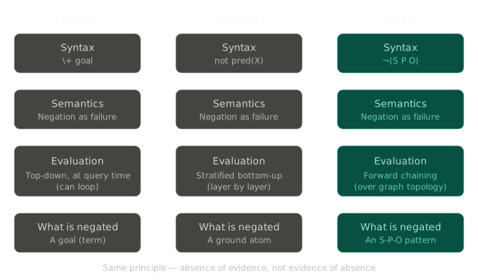
Negation in zelph follows negation-as-failure (NAF) semantics, familiar from Datalog with stratified negation and Prolog's \+. A negated condition succeeds when no fact in the graph matches the pattern under the current variable bindings.

The idiomatic syntax uses ¬:

zelph> (A is yellow, ¬(A is green)) => (A "is not" green)
zelph> plant is green
zelph> plant is yellow
zelph> plant2 is yellow
(plant2 "is not" green) ⇐ {(plant2 is yellow) (¬(plant2 is green))}

plant is both yellow and green, so ¬(plant is green) fails and the rule does not fire for plant. plant2 is yellow but not green, so the rule fires.

Negation is particularly powerful for structural queries — finding elements that lack a specific connection:

zelph> elem1 --> elem2
zelph> elem2 --> elem3
zelph> elem3 --> elem4
zelph> elem4 --> elem5
zelph> elem1 partoflist mylist
zelph> elem2 partoflist mylist
zelph> elem3 partoflist mylist
zelph> elem4 partoflist mylist
zelph> elem5 partoflist mylist
zelph> (A partoflist L, ¬(A --> X)) => (A "is last of" L)
(elem5 "is last of" mylist) ⇐ {(elem5 partoflist mylist) (¬(elem5 --> X))}

The negated condition ¬(A --> X) succeeds only when A has no outgoing --> link — identifying the last element purely declaratively.

A free variable inside ¬ is quantified inside it. Whichever position it stands in, the condition succeeds exactly when no fact matches — the free variable produces no binding that leaves the rule. So the same graph answers both directions the way their names suggest:

zelph> a ~ interval
zelph> b ~ interval
zelph> c ~ interval
zelph> a before b
zelph> b before c
zelph> (A ~ interval, ¬(A before B)) => (A is latest)
(c is latest) ⇐ {(¬(c before B)) (c ~ interval)}
zelph> (A ~ interval, ¬(B before A)) => (A is earliest)
(a is earliest) ⇐ {(a ~ interval) (¬(B before a))}

Datalog would refuse both rules outright: there, a variable under negation must be bound by a positive condition (range restriction), and B is not. zelph accepts them and gives them the reading the notation suggests.

Ranging over a domain is a positive condition, not a negation. To conclude something for each member of a set that lacks a property, name the set:

(X flagged S, ¬(X flagged bad)) => (X unflagged ok)

X flagged S is what makes an entity a candidate, and it says which candidates — the negation then only filters. The justification of each derived fact names both, so a result can be traced back to why the entity was considered at all.

The explicit (ASCII-only) equivalent of ¬(pattern) is *(pattern) ~ negation, using the focus operator *.

What ¬ applies to. A single fact pattern, not a group of them — ¬(A is y, A is z) is rejected rather than guessed at. Use De Morgan: ¬(A ∧ B) is (¬A) ∨ (¬B), and a disjunction is written as several rules with the same consequence:

(A is x, ¬(A is y)) => (A r s)
(A is x, ¬(A is z)) => (A r s)

Negating a group directly is an open direction, not a decision against it — see Where the logic goes next.

Where ¬ may stand, and what it means there. In a rule condition it is the negation-as-failure operator above. Alone on a line it is a claim: the fact does not hold.

zelph> ¬(a p b)
zelph> c p d
zelph> S p O
Answer: c p d

The refuted fact answers nothing, no rule fires on it, and zelph/exists reports it as absent – but it is not absent, it is denied. Asserting it afterwards is refused rather than silently overwritten, and so is refuting something the graph already claims:

zelph> ¬(a p b)
zelph> a p b
Error in line "a p b": fact(): this fact is known to be wrong

This is the mechanism zelph uses for a negative claim: a fact carries a probability, and one below 0.5 makes it known-wrong. The claim survives .save and .load, and it prints as what it is – the echo of ¬(a p b) is ¬(a p b), not a p b.

That reading belongs to the line, not to the prefix, so it does not extend to a statement that merely contains a pattern. There ¬ is refused:

zelph> x mentions (¬(a p b))
Error in line "x mentions (¬(a p b))": "¬" is a condition operator and has no meaning inside a plain statement: it succeeds when a pattern is ABSENT, which only a rule condition can ask. On its own line "¬(a p b)" says that the fact does not hold.

The marking a refutation writes is printed without the prefix for the same reason – (a p b) ~ refuted – since the predicate is already saying it, and a ¬ inside the subject would be interpreted as the condition operator when the line is re-entered.

A rule derives what holds, so a negated consequence still has no reading and is refused:

zelph> (A p B) => ¬(A q B)
Error in line "(A p B) => ¬(A q B)": "¬" is a condition operator and has no meaning as a consequence: a rule derives what holds, not what does not. To say that the two may not hold together, write a contradiction rule -- "(A p B, A q B) => !".

The contradiction rule the message names is what "these two must not hold together" is written as.

The other two condition operators have no reading outside a condition at all, and say so. ≈ asks what a network believes and ⁺ / ∗ ask what the engine can walk to; neither is something a line can assert. A path marker whose two ends are both concrete is refused, while the same shape with a variable in it is an ordinary question:

zelph> a P279 b
zelph> b P279 c
zelph> c P279 d
zelph> a P279⁺ d
Error in line "a P279⁺ d": "⁺" and "∗" are condition operators: reachability is what the engine WALKS, not what you assert. Write a variable to ASK ("S p⁺ b"), or use the path condition in a rule.
zelph> S P279⁺ d
(S P279 d) closure one-or-more
Answer: (a P279 d) closure one-or-more
Answer: (b P279 d) closure one-or-more
Answer: (c P279 d) closure one-or-more

Writing ¬ in front makes no difference to that. ¬(F) denies a fact, and neither of these two is one – there is no claim of reachability, or of what a net believes, for a line to deny:

zelph> ¬(a P279⁺ d)
Error in line "¬(a P279⁺ d)": "⁺" and "∗" are condition operators, and a "¬" in front does not change that: reachability is what the engine WALKS, so there is no claim of it to deny. Use the path condition in a rule, under "¬" if what you want is the absence of a path.
zelph> ¬≈net(a p b)
Error in line "¬≈net(a p b)": "≈" is a condition operator, and a "¬" in front does not change that: it asks what a network believes, which a rule condition can read and a statement can neither claim nor deny. Use it in a rule condition, under "¬" for the case the net does not confirm.

Nor does putting them one argument down. A plain statement has no condition slot at any depth, so all three operators are refused inside one:

zelph> x mentions (≈net(a p b))
Error in line "x mentions (≈net(a p b))": "≈" is a condition operator and has no meaning inside a plain statement: it asks what a network believes, which a rule condition can read and a statement cannot claim. Use it in a rule condition.
zelph> x mentions (a P279⁺ d)
Error in line "x mentions (a P279⁺ d)": "⁺" and "∗" are condition operators and have no meaning inside a plain statement: reachability is what the engine WALKS. On its own line "S p⁺ b" is a question and answers one; inside a rule it is a condition.

Under ¬ in a rule condition both are ordinary tests, which is the next section.

Inside a rule the three do have slots – but the slot is a whole condition, and an operator one argument further in is read by nothing. It is refused there too, in a condition and in a consequence alike:

zelph> (x q (¬(a p b))) => (c r d)
Error in line "(x q (¬(a p b))) => (c r d)": "¬" applies to a whole condition, not to something inside one: the tag it writes is read where the condition is, and nowhere below it. Write it in front of the condition -- "(A q B, ¬(A p B)) => ...".
zelph> (A p B) => (x q (a P279⁺ d))
Error in line "(A p B) => (x q (a P279⁺ d))": "⁺" and "∗" mark the predicate of a CONDITION, not of a fact inside one: the closure is walked for the condition itself, and a marker below it tags a fact nothing ever walks. Write the path as its own condition.

An inner rule is a rule, so a rule generator writing (P lifts Q) => ((X P Y, ¬(X Q Y)) => (X flagged Y)) is untouched by this: the ¬ there stands at the top of the inner rule’s own condition.

What ¬ may be applied to among the guards. Three conditions are not fact lookups but procedures the engine runs: the inequality guard !=, the neural condition ≈, and the path condition ⁺ / ∗. Two of them read under ¬ and one does not.

¬(C P⁺ T) and ¬≈net(S P O) are tests: the first succeeds when there is no path, the second when the net does not confirm the fact. Both need every term bound, because a negation binds nothing, and both say so when a term is open.

¬(X != Y) is rejected. It asks for the two terms to be the same node, and writing the same variable twice already asks that – with the advantage that the engine then uses it to narrow the search rather than testing afterwards:

The refusal comes when the rule is evaluated, not when it is read: != is a guard the engine runs, so what is rejected is the negation of that execution, and until a fact reaches the rule there is nothing to run.

zelph> (A prop X, A prop Y, ¬(X != Y)) => (A pair X)
((A prop Y), ¬(X != Y), (A prop X)) => (A pair X)
zelph> a prop v1
Error: ¬ cannot be applied to "!=" -- write the same variable on both sides to require two terms to be equal.

Stratified Evaluation

A negated condition asks about absence — but absence when? During a reasoning run, facts are still being derived; a negation evaluated mid-run could succeed merely because the matching fact had not been derived yet, and by monotonicity the resulting deduction could never be retracted. zelph therefore evaluates rules in strata:

1. Positive stratum: all rules without negated conditions run to quiescence (fixpoint).
2. Deferred stratum: rules whose conditions contain a negation at any nesting depth are evaluated against that saturated state.

Consequences of deferred rules may feed positive rules, so the two phases alternate until neither derives anything. This schedule is what makes negation-as-failure sound in a forward chainer: facts only accumulate, so a later derivation can make a negation fail but never make it newly succeed — a negation that succeeds at a stratum boundary is final. Both evaluation strategies (classic and semi-naive) implement the same schedule, and the .semi-naive check mode verifies their equivalence. How this check anchors engine development is described in Internals: Measurement Methodology.

The payoff is that universally quantified conditions can be written the way a textbook would state them. The primality rule

(N testprime N, &2 < N, ¬(N hasdivisor D)) => (N isprime N)

is sound as written: it is deferred until every divisor candidate has been tested, so the negation quantifies over the complete scan. See Semantic Arithmetic for the full module.

Two boundaries are worth knowing:

• One negation stratum. If a deferred rule's consequences can (transitively) grow the extension of a pattern negated by another deferred rule, the program is not stratifiable in a single layer, and results within the deferred phase may depend on rule order. Contradiction rules (consequence !) are always safe here: they derive no facts.
• Stratification orders derived facts, not your input. Negation is evaluated per run, against asserted facts as they stand. If a negated pattern should be blocked by base facts, assert those facts before the triggering fact.

Inequality Constraints

🎬 Watch this section

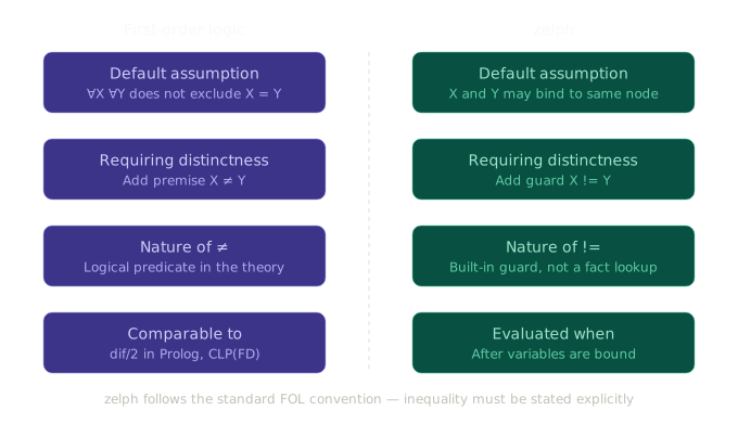
The != operator is a built-in guard constraint — not a fact lookup. It filters variable bindings after the involved variables are bound by positive conditions.

Key design decision: In zelph, two different variable names may bind to the same node. This is consistent with standard first-order logic where ∀x ∀y. P(x,y) does not exclude x = y. To require distinct bindings, an explicit != constraint is needed.

zelph> (A prop X, A prop Y, X != Y) => (A has_pair X Y)
zelph> a prop v

With only one value v, the binding X = v, Y = v is blocked by !=, so the rule does not fire.

zelph> a prop v1
(a has_pair v v1) ⇐ {(a prop v) (v1 != v) (a prop v1)}
zelph> a prop v2
(a has_pair v v2) ⇐ {(a prop v2) (v != v2) (a prop v)}
(a has_pair v1 v2) ⇐ {(a prop v2) (v1 != v2) (a prop v1)}

Once distinct values exist, the rule fires for the distinct pairings – for every one of them, v included, since it too differs from the new values.

Practical use case — detecting functional-property violations (a pattern from Wikidata ontology work):

zelph> (P is functional, A P X, A P Y, X != Y) => !
zelph> date_of_birth is functional
zelph> alice date_of_birth 1990
zelph> alice date_of_birth 1991
! ⇐ {(alice date_of_birth 1990) (alice date_of_birth 1991) (date_of_birth is functional) (1991 != 1990)}
Found one or more contradictions!

Without !=, the rule would also fire when the same value is entered redundantly, which is not a real conflict.

Why != matters — preventing spurious deductions:

Without !=, rules that quantify over pairs can produce false positives from reflexive bindings:

(X opposite Y, A ~ X, A ~ Y) => !
bright opposite bright
yellow ~ bright

Without !=, the engine binds X = bright, Y = bright, satisfies all conditions, and fires the contradiction — even though yellow is merely classified under the same category twice. Adding X != Y blocks this reflexive binding and prevents the false positive.

Constraint checking — Graph coloring:

Multiple != constraints can enforce pairwise distinctness, enabling constraint-checking patterns:

zelph> (A adjacent B, A color X, B color X) => !
zelph> r1 adjacent r2
zelph> r2 adjacent r3
zelph> r1 color red
zelph> r2 color blue
zelph> r3 color red

No contradiction — the coloring is valid. But assigning r2 color red instead would trigger the contradiction, since adjacent regions r1 and r2 would share the same color.

Self-joins: derive the selection first

A rule that pairs a relation with itself is quadratic in that relation, and != does not make it cheaper — the guard filters bindings after the join has produced them. When the pairs you actually want are a small subset picked out by other conditions, deriving that subset first and joining over it is the same statement in a far cheaper order:

# quadratic over every `hits` fact, then filtered
(A hits B, A hits C, B != C, B holds K, K ~ valuable, C holds L, L ~ valuable)
    => (A ~ double_attacker)

# the selection pushed below the join
(A hits B, B holds K, K ~ valuable) => (A threatens B)
(A threatens B, A threatens C, B != C) => (A ~ double_attacker)

Both derive the same facts. On a base of ~200 facts in which about 60 were hits and 8 of those were threats, the two-rule form ran 14× faster — and the whole rule set it belonged to went from 4.07 ms to 0.96 ms.

The reason is worth knowing, because it tells you when to expect this. optimize_order plans the join by boundness: a condition whose subject and objects are already bound scores higher, because unification can resolve it without scanning. It does not know how many facts a relation has, and cannot — that is a property of the data, not of the rule. So the planner can put a resolvable condition first, but it cannot tell a scan over 60 facts from a scan over 8. Where a relation's size is what makes one order cheap, the rule author supplies that knowledge by naming the smaller relation.

The same reasoning applies to a negated condition or an ≈ condition inside a self-join: both are evaluated per candidate binding, so anything that shrinks the candidate set first pays for itself.

"Is this the only one?"

A derived marker also answers the question that looks as if it needed a negation over a conjunction — ¬(A prop Y, X != Y), which is not expressible. Derive the positive case with the guard, then negate that single pattern:

zelph> b prop w
zelph> a prop v1
zelph> a prop v2
zelph> (A prop X, A prop Y, X != Y) => (A ~ several)
(a ~ several) ⇐ {(v2 != v1) (a prop v1) (a prop v2)}
zelph> (A prop X, ¬(A ~ several)) => (X ~ sole)
(w ~ sole) ⇐ {(¬(b ~ several)) (b prop w)}

Note the order: the facts come before the rules. Negation is evaluated per run against the facts as they stand, and the graph is monotonic — with a prop v1 alone in the graph, the second rule derives v1 ~ sole, and a prop v2 arriving later cannot take that back.

Fresh Variables: Generative Rules

Variables that appear only in the consequence of a rule are treated as fresh: the engine generates new anonymous nodes for them during inference.

zelph> .deductions all
Deduction printing mode: all
zelph> (A is human) => (B nameof A)
zelph> tim is human
(?? nameof tim) ⇐ (tim is human)
zelph> X nameof tim
Answer: ?? nameof tim

The ?? represents a newly created node — an existential witness materialized in the graph. It is the same node in both lines; a node the engine generated has no name to print.

.deductions all is needed here and is not decoration. The default mode is focus, which prints a deduction only when its subject came from something you entered (reference) — and the subject of a generative rule's consequence is the generated node itself, which by definition never did. The fact is derived and stored either way; only the line announcing it is suppressed.

Termination guarantee: Before creating a new node, zelph checks whether the deduced facts (with the fresh variable as wildcard) already exist. If they do, no new deduction occurs. This ensures that generative rules converge.

This mechanism is fundamental for constructive reasoning, such as building new cons-list structures during arithmetic (see below).

A Predicate Logic Perspective

For readers with a background in formal logic, here is how zelph's constructs map to first-order logic.

Universal Quantification

Variables in rule conditions behave like universally quantified variables. The transitive-closure rule

(R ~ transitive, X R Y, Y R Z) => (X R Z)

reads as:

\[ \forall R\, \forall X\, \forall Y\, \forall Z.\; \bigl(\text{transitive}(R) \wedge R(X,Y) \wedge R(Y,Z)\bigr) \to R(X,Z) \]

with the caveat that quantification ranges over the current fact base (closed-world evaluation), not over all possible interpretations.

Existential Quantification

Fresh variables (those appearing only in the consequence) correspond to constructive existential quantification. In Skolem-function terms, each fresh variable is implicitly Skolemized relative to the universally quantified condition variables.

Conjunction

The comma-separated condition syntax (cond1, cond2, cond3) is a conjunction: all conditions must match under a shared variable assignment. The conditions are evaluated as a joint constraint (the semantics are order-independent, even if the engine may internally choose an evaluation order for efficiency).

Negation

¬(Pattern) corresponds to negation-as-failure (NAF) — the same semantics as in Datalog with stratified negation or Prolog's \+. It tests the absence of evidence in the current graph state, not the evidence of absence in the model-theoretic sense. Readers familiar with Answer Set Programming (ASP) or well-founded semantics will recognize this as a form of default negation operating over the graph's Herbrand base. zelph enforces these semantics operationally by deferring rules with negated conditions until the positive rules reach their fixpoint (see Stratified Evaluation).

Inequality

The != operator corresponds to dif/2 in Prolog or disequality constraints in CLP(FD). It is a guard, not a fact pattern.

Disjunction

zelph currently supports conjunction but not explicit disjunction in rule conditions. As in Datalog, disjunction is expressed through multiple rules with the same consequence pattern:

(A is bird) => (A can fly)
(A is bat) => (A can fly)

This is equivalent to (bird(A) ∨ bat(A)) → can_fly(A).

When both branches hold, the consequence is derived once, not twice: a fact is a node and nodes are hash-consed, so the second rule finds the fact the first one made. A query therefore answers a doubly-justified conclusion exactly once.

Unary Predicates and Self-Facts

zelph facts are subject–predicate–object triples; there is no dedicated arity-1 fact form. A unary predicate P(x) is therefore expressed as a self-fact — a fact whose subject and object are the same node:

x P x

The term is zelph's own coinage; in graph-theoretic terms a self-fact is a loop at x, in relational terms it places x on the diagonal of the binary relation P — asserting P(x) via x P x is the classic encoding of unary predicates in a formalism whose primitive is a binary relation. The standard library uses self-facts as request markers: (N testprime N) triggers the primality test, (T simplify T) a simplification. The self-fact prefix : makes both directions convenient — :testprime N on input, and the same compact form on output.

A natural question, especially from a mathematical perspective: why not assign every operator a fixed arity — simplify unary, + binary — so that simplify(T) is primitive and no marker encoding is needed? The answer is the first-class-predicate design discussed above: a predicate in zelph is an ordinary node without a signature. The node + is not exclusively an operator. The fact (&2 + &3) is itself a node that appears as the subject of the result fact ((&2 + &3) = &5); meta-rules quantify over predicates (R is transitive); and facts may carry several objects, so even "binary" is not structurally fixed. A schema layer assigning arities would have to constrain exactly the flexibility that makes meta-rules expressible. Consequently, whether a predicate acts as a term-forming operator or as a marker is knowledge of the module that defines it, not of the engine — which is why the corresponding display decision is a script-level declaration (zelph/no-selffact-sugar, the same philosophy as zelph/number), not a built-in rule.

Semantic Math: Computation as Graph Rewriting

🎬 Watch this section

Numbers in zelph are not opaque primitives. They are cons-lists of digit nodes — topological structures within the graph, built from the same cons and nil predicates used for any list. Arithmetic is not hard-coded; it is defined by inference rules that transform these structures.

This architecture has a remarkable consequence: calculating numbers and reasoning about numbers happen in the same system. If a knowledge base (e.g. Wikidata) records that 13 is a prime number, that semantic fact is directly accessible wherever the list <13> appears in a computation.

Numbers as Cons-Lists

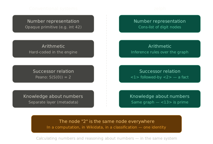
The list <42> is internally stored as 2 cons (4 cons nil) — least significant digit first. The display reverses the order for human readability, so results appear in conventional notation. For details on the list syntax, see Angle Brackets: Lists.

This representation means digits are ordinary named nodes. The node "4" is the same node everywhere in the graph — in a number, in a Wikidata entity, in a classification.

Peano-style Successor Addition

The simplest possible addition rule uses a successor table:

zelph> <0> followed-by <1>
zelph> <1> followed-by <2>
zelph> <2> followed-by <3>
zelph> (A followed-by B) => ((<1> + A) = B)
((<1> + <0>) = <1>) ⇐ (<0> followed-by <1>)
((<1> + <2>) = <3>) ⇐ (<2> followed-by <3>)
((:+ <1>) = <2>) ⇐ (<1> followed-by <2>)

This states: if A is followed by B in the number succession, then 1 + A = B. The engine derives one sum per successor fact, and it derives them in whatever order the run reaches them. (<1> + <1>) = <2> is among them: subject and object of the sum coincide there, so it is printed with the self-fact prefix as (:+ <1>) = <2>, which re-enters as the same fact.

The key point: followed-by is a user-defined relation. zelph has no arithmetic kernel. The rule works because the graph contains the corresponding facts.

Rule-based Multi-digit Addition

🎬 Watch this section

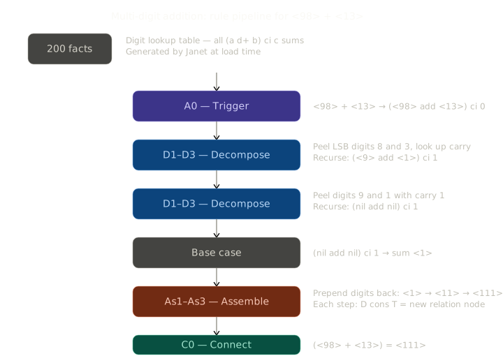
Deep dive: this section develops the addition module as a proof of concept. The dedicated page Semantic Arithmetic covers the full arithmetic system — subtraction, comparison, and multiplication — the shared architecture behind all four rule modules, the base-independence property, and the engine machinery (bound-pattern grounding, semi-naive evaluation) that makes rule-based computation fast.

zelph can perform arbitrary-precision addition purely via graph rules. The reference implementation lives in stdlib/decimal-arithmetic.zph. A second reference implementation, stdlib/binary-arithmetic.zph, performs the same computation in base 2. Because the digit-level knowledge shrinks to the 16 hand-written facts of a full adder truth table, it needs no generated lookup table at all — apart from its zelph/number definition, it is written in pure native zelph syntax, without the Janet API. The recursion rules are identical in both scripts: they are base-agnostic, which nicely demonstrates that the base is a property of the data, not of the rules.

The algorithm consists of three parts:

1. A digit-level lookup table (generated programmatically via Janet):

For all digits a,b ∈ {0..9} and carry-in c ∈ {0,1}, two facts encode the sum and carry-out:

• ((a d+ b) ci c) sum s where s = (a + b + c) mod 10
• ((a d+ b) ci c) co e where e = ⌊(a + b + c) / 10⌋

This turns digit arithmetic into ordinary facts in the network — 200 entries total.

2. Base cases for the recursion endpoint (when both operands are nil):

• ((nil add nil) ci 0) sum nil
• ((nil add nil) ci 1) sum <1>

3. Eight inference rules that decompose, propagate carries, assemble results, and connect to the user-facing = predicate.

The rules handle three cases each for decomposition (both operands non-nil, left nil, right nil) and assembly, plus a trigger rule and a connection rule.

A Worked Example

Note: since decimal-arithmetic.zph registers its digit alphabet, a live session displays these lists as decimal &-literals (e.g. &12345 instead of <12345>).

The intermediate states below are shown with .deductions all. The default mode (focus) derives them all the same but prints only the final = fact — see Deduction Output Modes.

.import decimal-arithmetic
(<12345> + <98765>) = X

Trigger (Rule A0): Seeds the internal addition state with carry-in 0:

((&12345  add  &98765)  ci   0 )

Decomposition (Rules D1–D3): Peels off least-significant digits, propagates carry:

((&1234  add  &9876)  ci   1 )
((&123  add  &987)  ci   1 )
((&12  add  &98)  ci   1 )
((&1  add  &9)  ci   1 )

Base case: The recursion ends at nil + nil with carry-in 1:

((( nil   add   nil )  ci   1 )  sum  &1)

Assembly (Rules As1–As3): Constructs the result on the way back up, prepending digits via cons:

(((&1  add  &9)  ci   1 )  sum  &11)
(((&12  add  &98)  ci   1 )  sum  &111)
...
(((&12345  add  &98765)  ci   0 )  sum  &111110)

Connection (Rule C0): Exposes the result under the user-facing = predicate:

((&12345  +  &98765)  =  &111110)

Nothing in the engine is hard-coded for addition. The computation emerges from the same topological primitives used for ordinary knowledge representation — facts, conjunctions, cons-lists — plus eight generic inference rules.

Asserting vs. Querying

&123456 + &987654 is an assertion, not a query: it adds the + fact to the graph, and the inference engine derives the result (plus all intermediate add/ci/sum states) exactly once. Re-entering the same assertion produces no output -- the fixpoint has already been reached, which is correct forward-chaining behaviour. To retrieve a result (again), use a query:

(&123456 + &987654) = X

Queries contain variables and are always evaluated, so this prints the result no matter how often it is repeated. The derived intermediate facts deliberately stay in the graph: they are reusable knowledge for subsequent computations. To sandbox a computation instead, wrap it in a cluster and drop it afterwards.

By default, the REPL's deduction trace is filtered to facts about your input; see Deduction Output Modes.

Semantic Integration with Knowledge Graphs

Because list elements are ordinary graph nodes, any arithmetic rule that produces a digit automatically inherits all semantic facts known about that digit. If the Wikidata graph is loaded, querying all prime numbers is a standard pattern query:

.lang wikidata
X P31 Q49008

This lists all 10,018 prime numbers recorded in Wikidata — the same nodes that would appear in a cons-list produced by arithmetic rules. Knowledge and computation are not separate layers.

Comparison and Subtraction

The addition pattern generalizes: both arithmetic scripts also define comparison and subtraction, and the recursion rules are again byte-identical between the decimal and binary script — only the digit tables differ (100/400 generated facts in base 10, 4/16 hand-written facts in base 2; the subtraction table is the truth table of a full subtractor).

Comparison (N cmp M) walks both lists LSB-first and combines a digit table (dcmp) with a dominance rule: the more significant rest decides unless it is eq, in which case the current digit pair decides. Missing digits are zero-extended, so lists with leading zeros compare correctly by value. The results are ordinary relational facts — N < M, N > M, N == M — and therefore compose with meta-rules like any declared fact:

(R is transitive, A R B, B R C) => (A R C)
> is transitive
&30 cmp &20
(&30 > &20) ⇐ {((&30 lcmp &20) res gt) (&30 cmp &20)}
&20 cmp &10
(&20 > &10) ⇐ {((&20 lcmp &10) res gt) (&20 cmp &10)}
(&30 > &10) ⇐ {(&30 > &20) (> is transitive) (&20 > &10)}

Computed order and declared knowledge feed the same inference engine.

Additionally, the outcome is exposed under = for uniform result queries: (A cmp B) = X answers gt/lt/eq.

Subtraction (N - M) mirrors addition exactly, with borrow (bi/bo) instead of carry. It is deliberately a partial function on the naturals: if M > N, the borrow chain reaches the base case with borrow-in 1, for which no base fact exists — the derivation simply produces no result. Undefinedness is encoded as the absence of a fact; no error machinery is involved.

Non-canonical results: subtraction can yield lists with leading zeros (&105 - &98 produces the list <007>). The &-display normalizes the value (&7), and comparison treats such lists as equal by value — but they remain distinct nodes. Operands are expected in the canonical form produced by &-literals.

Multiplication: Cross-Module Computation

Multiplication completes the picture and introduces a new structural element: rules that delegate to other rule modules. The recursion runs over the first operand's digits — (A cons R) × M = A×M + base × (R×M) — and because numbers are stored LSB-first, multiplying by the base is a single cons: base × X = (0 cons X). No shift machinery exists; it falls out of the representation.

The digit-times-number products use a third digit table (dx, with running carry — 1800 generated facts in base 10, 16 hand-written facts in base 2: an AND gate plus increment, completing the full-adder/full-subtractor family). The accumulation, however, is not implemented in the multiplication module at all: rule MA1 asserts an ordinary + fact, the addition module derives its = result through its own rules, and rule MA2 consumes it. Computation cascades across modules through nothing but shared facts — the same mechanism that lets computed comparison facts feed declared meta-rules.

As with the other operations, the recursion rules are byte-identical between the decimal and the binary script. Since intermediate states are hash-consed graph nodes, partial products that share suffixes are shared automatically — memoization is a property of the representation, not a feature.

A schema note for rule authors: all three digit tables are keyed by dedicated table-carry predicates (tci for the addition and multiplication tables, tbi for subtraction) while recursion states use ci/bi/mci. Keeping table space and state space on distinct predicates ensures tables are only ever accessed through direct, grounded lookups and never appear in the extensions scanned when a rule's first condition is matched -- those extensions then contain nothing but the small, dynamic recursion states. Sharing tci between two tables is deliberately harmless: table-keying predicates are never scanned.

Division and remainder complete the four operations; see Semantic Arithmetic for the candidate-selection design.

Number Literals

Cons-lists are a general-purpose structure — numbers are merely one use of them, and zelph deliberately does not hard-code any numeric representation. Which base is used, or whether digits are decimal characters at all, is decided entirely by the loaded rule scripts. The parser, however, offers two pieces of syntax sugar that make the numeric use case pleasant without constraining it:

1. Inverting angle brackets. Compact lists like <123> reverse their characters before cons construction, so the least significant digit becomes the outermost cell — the natural orientation for right-to-left arithmetic rules (see Angle Brackets: Lists).

2. The & prefix. A token like &42 is always decimal input, regardless of the internal representation. The parser transforms it into (zelph/number "42") — a call to the redefinable Janet function zelph/number, whose default implementation raises an error until a representation is loaded. stdlib/decimal-arithmetic.zph maps it to a decimal digit list (&42 ≡ <42>), while stdlib/binary-arithmetic.zph converts to base 2 (&5 ≡ <101>). The prefix applies unconditionally: a token starting with & is a number literal, and if the loaded zelph/number cannot interpret it, that is an error — by design, there is no silent fallback to an atom. Every stdlib substrate reads the literal the same way, which is what makes them interchangeable under the shared module ID arithmetic: non-digits are rejected (&abc is an error, not a cons list of letters), and leading zeros are stripped, so &007 and &7 denote the same node. (The choice of & is a small homage to classic home-computer BASICs, where & prefixed number literals.)

3. Symmetric output. The display side mirrors the input side: a script can register its digit alphabet via (zelph/set-number-digits ["0" "1" ...]) (digit nodes or names, in ascending order of value). From then on, node_to_string renders every properly nil-terminated cons list that consists solely of registered digit nodes as a decimal &-literal -- regardless of the internal base. stdlib/decimal-arithmetic.zph registers 0–9, stdlib/binary-arithmetic.zph registers 0 and 1, so both display &5 for their respective internal lists <5> and <101>. Any other cons list -- including lists of single-character nodes that are not registered digits -- keeps the generic <...> display, so cons lists remain general-purpose. An empty array disables the feature.

This split keeps the philosophy intact: the representation of numbers lives in scripts and rules, while the convenience of familiar decimal input lives in the parser — decoupled through one redefinable function.

Beyond Arithmetic

The techniques demonstrated by the addition algorithm — deep unification, recursive decomposition via cons-lists, fresh variable generation, and digit-level lookup tables — are general-purpose. They apply whenever computation can be expressed as structure transformation over a graph.

Statements About Statements

Because fact nodes can themselves appear as subjects or objects, zelph naturally supports higher-order assertions. For example, declaring a relation to be symmetric, transitive, or functional is a statement about a predicate — and the inference engine treats it as an ordinary fact that conditions can match against.

This enables concise, generic rules that would require meta-interpreters or reflection mechanisms in traditional logic programming systems.

Neural Rule Conditions

Since version 0.9.7, rule conditions can also consult a neural network living inside the same graph, via the ≈ operator — verifying facts against a learned model (guard mode) or generating candidate bindings above a confidence threshold (generator mode), with the confidence flowing into the deduced fact's probability. This neuro-symbolic capability has its own page: Neural Networks in the Graph.

Transitive Path Conditions

A condition may follow a predicate any number of steps instead of exactly one. Suffix the predicate with ⁺ (U+207A) for one or more steps, or with ∗ (U+2217) for zero or more:

zelph> Q1 P279 Q2
zelph> Q2 P279 Q3
zelph> Q3 P279 Q4
zelph> alice member Q1
zelph> (X member C, C P279⁺ T) => (X "belongs to" T)
(((C P279 T) closure one-or-more), (X member C)) => (X "belongs to" T)
(alice "belongs to" Q2) ⇐ {((Q1 P279 Q2) closure one-or-more) (alice member Q1)}
(alice "belongs to" Q3) ⇐ {((Q1 P279 Q3) closure one-or-more) (alice member Q1)}
(alice "belongs to" Q4) ⇐ {((Q1 P279 Q4) closure one-or-more) (alice member Q1)}

C is bound by the first condition, so the path condition walks forward from Q1 and produces one binding for T per class reached. With the target bound instead, it walks backward; with both ends bound it is a reachability test that filters rather than generates. Reachability is answered by the same indexed closure engine that zelph/closure and the SPARQL layer's p+ / p* use — built once per predicate and cached next to the .bin, not walked per query.

Both ends free is refused, with a message asking you to bind one: a path over an unanchored pair would enumerate every path in the graph. The condition is scheduled after the conditions that bind ordinary variables, so the order in which you write it does not matter. The predicate itself must be a concrete predicate — a closure is indexed per predicate, and quantifying over predicates remains the business of an ordinary condition, which can do it.

The operator is not a reserved character. It is read only as a trailing marker in predicate position, and only when a name is left over once it is removed, so Na⁺ is an ordinary node name in any position, a⁺b is an ordinary predicate, and ⁺ on its own is the predicate ⁺. ASCII + deliberately has no such reading, because z+ and d+ are the addition predicates of the arithmetic modules, and * is the focus operator.

Like ≈, the sugar is input syntax over an ordinary fact: (C P279⁺ T) is the fact ((C P279 T) closure one-or-more), which is what .list-rules prints and what re-enters as the same rule.

A marker on a self-fact inquires if a node reaches itself, since :pred X is (X pred X) and predicate position is where the marker is read. That is a cycle test, and it needs nothing beyond what is already here – one condition to bind the node, and the path condition to ask:

zelph> Q1 ~ class
zelph> Q2 ~ class
zelph> Q5 ~ class
zelph> Q1 P279 Q2
zelph> Q2 P279 Q1
zelph> Q5 P279 Q6
zelph> (C ~ class, :P279⁺ C) => (C "sits in a cycle" C)
((C ~ class), ((:P279 C) closure one-or-more)) => (C "sits in a cycle" C)
(Q1 "sits in a cycle" Q1) ⇐ {(Q1 ~ class) ((:P279 Q1) closure one-or-more)}
(Q2 "sits in a cycle" Q2) ⇐ {(Q2 ~ class) ((:P279 Q2) closure one-or-more)}

Q5 is excluded: it has a superclass, but no path back to itself. With ∗ every node qualifies instead, since zero steps is a path.

Under ¬ the condition asks the same question the other way round: does this node not reach that one.

zelph> Q1 P279 Q2
zelph> Q2 P279 Q3
zelph> Q4 P279 Q9
zelph> alice member Q1
zelph> bob member Q4
zelph> (X member C, ¬(C P279⁺ Q3)) => (X clear-of Q3)
(bob clear-of Q3) ⇐ {(bob member Q4) (¬((Q4 P279 Q3) closure one-or-more))}

alice is excluded since Q1 reaches Q3 in two steps. A negated path condition requires both ends bound, and it reports it otherwise: the affirmative version accepts one bound endpoint and produces the other, but a negation binds nothing, thus there is nothing for an open endpoint to transform into. "Reaches nothing at all" poses a distinct inquiry, and it is asked by binding the far end.

The cost operates in reverse as well, and it is important to recognize prior to crafting one for a large graph. The positive form walks the closure once from the bound end. The negated form involves a test for each candidate, so a rule whose other conditions leave thousands of candidates incurs one reachability walk for each of them. Where the inquiry is genuinely a set difference over one predicate – every class below A that is not below B – the SPARQL layer's MINUS computes the two closures once and subtracts, which is the shape to reach for at that scale.

A result derived through a path condition stays reconstructible. .explain marks the walked premise [closure] rather than [axiom], because nobody asserted the path — the engine walked it, and there is no fact to expand further:

zelph> .explain (alice "belongs to" Q4)
alice "belongs to" Q4
   ├─ alice member Q1  [axiom]
   └─ (Q1 P279 Q4) closure one-or-more  [closure]

Contradiction Detection

Rules with ! as the consequence detect logical inconsistencies:

zelph> (X "is opposite of" Y, A ~ X, A ~ Y, X != Y) => !
zelph> bright "is opposite of" dark
zelph> yellow ~ bright
zelph> yellow ~ dark
! ⇐ {(bright "is opposite of" dark) (yellow ~ bright) (bright != dark) (yellow ~ dark)}
Found one or more contradictions!

When a contradiction is detected during fact assertion, the contradictory fact is not entered into the graph. Instead, a record of the contradiction is stored, making it visible in reports. This mechanism is central to zelph's Wikidata ontology work, where thousands of constraint violations in the knowledge graph are detected automatically.

The record is a fact in the graph, and it says what a contradiction says: the set of the statements that matched, entered as refuted – these do not hold together. None of them is retracted; each stays asserted and keeps answering queries, and the set is the only node created.

That is also why a contradiction is announced once rather than on every later run. A set constant is identified by its members, so the same contradiction always yields the same node, and the next run finds it already there – the same way a derived fact stays quiet the second time because the graph holds it. Details, including the switch that turns the record off, are on the overview page and in .help .contradiction-records.

Silence differs from a clean graph, thus the summary of a run says which of the two applies. A network that already holds records reports them next to the count of what this run found: 0 contradictions found (1 already recorded in this network). The number is extracted from the graph rather than counted as the run meets them, so it counts contradictions and not the rule instantiations that reach them – a symmetric rule matches the same pair twice and still reports one. A network you downloaded therefore states what it holds on the very first run over it.

Wikidata at Scale

🎬 Watch this section

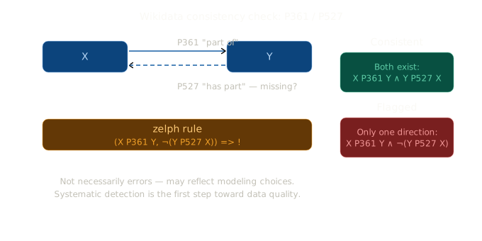
zelph can load and reason over millions of Wikidata facts. A typical consistency check uses negation to detect missing inverse relations:

.load wikidata-20260309-all-pruned-medium.bin
.lang wikidata
(X P361 Y, ¬(Y P527 X)) => !
.run

Here, P361 ("part of") and P527 ("has part") are inverse properties. The rule flags every entity declared "part of" something whose parent does not list it among its parts.

On wikidata-20260309-all-pruned-medium.bin this reports 355,073 contradictions from 547,551 unification matches, in five minutes of reasoning. How many a given network yields depends on which one – each published variant carries a different set of individual items – but the order of magnitude is the point: these are not a handful of stragglers. They are also not necessarily errors, since they may reflect deliberate modeling choices about redundancy; detecting them systematically is the first step toward improving data quality at scale. This is exactly the kind of analysis performed in the Wikidata Ontology Cleaning Task Force, supported by a Wikimedia Community Fund grant.

The Programmatic Layer: Janet

zelph embeds Janet, a lightweight functional programming language, as its scripting layer. Janet serves as a powerful macro system: it constructs graph structures that are then processed by zelph's reasoning engine. During inference, only zelph's native engine runs.

Janet is used for:

• Generating facts programmatically — e.g. the 200-entry digit addition lookup table is generated by a Janet loop, not entered manually.
• Parameterized rules — functions that create rule topologies for any relation.
• Querying and inspecting the graph — zelph/query returns results as Janet data structures.
• External integration — Janet's standard library provides file I/O, networking, and data processing, enabling zelph to exchange data with external systems.

For the full Janet API reference and examples, see the Janet scripting documentation.

A quick taste — generating a transitive rule for any relation:

%
(defn transitive-rule [rel]
  (zelph/rule
    [(zelph/fact 'X rel 'Y)
     (zelph/fact 'Y rel 'Z)]
    (zelph/fact 'X rel 'Z)))

(transitive-rule "is part of")
(transitive-rule "is ancestor of")
%

A single function call creates the entire rule topology — conjunction set, conditions, consequence, and the => link — for any named relation.

Getting Started

To try zelph yourself, see the Quick Start Guide for pre-compiled binaries on all major platforms. The interactive REPL lets you enter facts and rules and observe inference in real time — every example on this page can be entered directly.

The project is open source (AGPL v3 / commercial dual license) and hosted on GitHub.